load("_book/data/toydata.obj")4 Getting to grips with the mixed models
To illustrate the impact of variance components, the model choice, and impact on confidence intervals two very simple data sets has been purposefully constructed.
You can download the data sets here. They are stored as an single R object that contains both data sets. Download it to your computer.
You can get this download into your R session via (while providing the path that applies on your system):
We plot the data sets ds1 and ds2 sets to get an idea what they are about.
gridExtra::grid.arrange(
ggplot(ds1,aes(y=value,x=treatment,color=animal)) +
  geom_point(position = position_jitter(h=0,w=0.1),size=3,alpha=.7) +
  ylim(c(19,32)) + ggtitle("ds1"),
ggplot(ds2,aes(y=value,x=treatment,color=animal)) +
  geom_point(position = position_jitter(h=0,w=0.1),size=3,alpha=.7) +
  ylim(c(19,32)) + ggtitle("ds2"),
ncol=2
)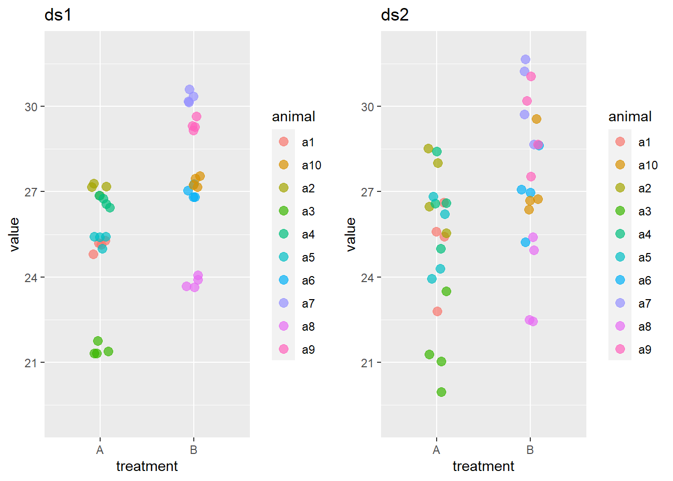
The effects are same in both data sets as can be checked by simple means. When generating the data an effect size of treatment B that was 2.5 units larger than the one of treatment A.
ds1 %>% group_by(treatment) %>% summarise(om=mean(value))# A tibble: 2 × 2
treatment om
<chr> <dbl>
1 A 25.1
2 B 27.6ds2 %>% group_by(treatment) %>% summarise(om=mean(value))# A tibble: 2 × 2
treatment om
<chr> <dbl>
1 A 25.1
2 B 27.6Both data sets contain measurements on 10 animals that were given either treatment A or treatment B. Four observations are made on each animal. The data are constructed such that the effects of the treatments and the average for each animal is the (approximately) the same in both data sets, despite the large difference in variation between the observations in each data sets.
4.1 Comparing fixed and mixed models
To demonstrate how the various model approaches differ, fit the naive fixed model, the fixed model on the averages by animal, and the mixed model with animal as random grouping effect to both data sets. Check the coefficients, the standard errors on these coefficients, and the degrees of freedom.
Comment on what you see.
Below some code to help if needed.
click to see the coding help
# naieve fixed models
lmi.ds1 <- lm(data=ds1,value~treatment)
lmi.ds2 <- lm(data=ds2,value~treatment)

# fixed models on average by animal
ds1.avg <- ds1 %>% group_by(animal,treatment) %>% summarise(value=mean(value))
ds2.avg <- ds2 %>% group_by(animal,treatment) %>% summarise(value=mean(value))

lma.ds1 <- lm(data=ds1.avg,value~treatment)
lma.ds2 <- lm(data=ds2.avg,value~treatment)

# mixed model by animal
library(lme4)

lmera.ds1 <- lmer(data=ds1,value~treatment + (1|animal))
lmera.ds2 <- lmer(data=ds2,value~treatment + (1|animal))

summary(lmi.ds1)$coefficients
summary(lmi.ds2)$coefficients
summary(lma.ds1)$coefficients
summary(lma.ds2)$coefficients
summary(lmera.ds1)$coefficients
summary(lmera.ds2)$coefficients
Now also calculate the confidence interval on the coefficient for treatment B (tip: use parm = "treatmentB" as argument in confint) and compare those for the three models.
click to see the coding help
ci.ds1 <- bind_rows(
  data.frame(model="1.lmi",confint(lmi.ds1,parm="treatmentB")),
  data.frame(model="2.lma",confint(lma.ds1,parm="treatmentB")),
  data.frame(model="3.lmera",confint(lmera.ds1,parm="treatmentB"))
) %>% rename(low = "X2.5..",up = "X97.5..")

ci.ds2 <- bind_rows(
  data.frame(model="1.lmi",confint(lmi.ds2,parm="treatmentB")),
  data.frame(model="2.lma",confint(lma.ds2,parm="treatmentB")),
  data.frame(model="3.lmera",confint(lmera.ds2,parm="treatmentB"))
) %>% rename(low = "X2.5..",up = "X97.5..")
The confidence intervals that you should have found look like this.
gridExtra::grid.arrange(
ci.ds1 %>% ggplot() + geom_errorbar(aes(x=model,ymin=low,ymax=up),width=.2) +
  ggtitle("ds1"),
ci.ds2 %>% ggplot() + geom_errorbar(aes(x=model,ymin=low,ymax=up),width=.2) +
  ggtitle("ds2"),
ncol=2)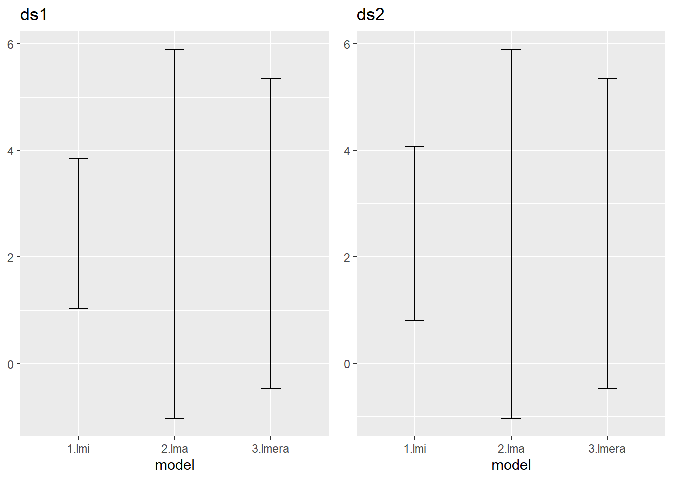
The interval of the mixed model is intermediate between the one obtained via the individual observation fixed model and the average base fixed model.
Try to explain
- why you get these three very different results.
- the difference between the outcome for both data sets
4.2 Another random effect
Suppose that the experiments existed of several replicates that contained each time two animals, one for treatment A and one for treatment B.
gridExtra::grid.arrange(
  ggplot(ds1,aes(y=value,x=treatment,color=as.factor(rep))) +
    geom_point(position = position_jitter(h=0,w=0.1),size=3,alpha=.7) +
    ylim(c(19,32)) + ggtitle("ds1"),
  ggplot(ds2,aes(y=value,x=treatment,color=as.factor(rep))) +
    geom_point(position = position_jitter(h=0,w=0.1),size=3,alpha=.7) +
    ylim(c(19,32)) + ggtitle("ds2"),
  ncol=2
)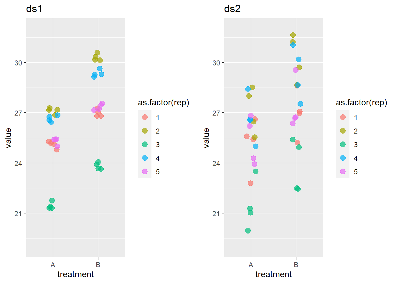
The graph, particularly in ds1, makes clear that there is a large replicate effect.
The mixed model needs to reflect that dependency. The random effect definition should now be + (1|rep/animal): observations are grouped within animals that are grouped within replicates. Because there is only one animal with a given treatment within each replicate, the (1|rep/animal) is in this case equivalent to (1|rep).
lmerr.ds1 <- lmer(data=ds1,value~treatment + (1|rep))
lmerr.ds2 <- lmer(data=ds2,value~treatment + (1|rep))

summary(lmerr.ds1)
Linear mixed model fit by REML ['lmerMod']
Formula: value ~ treatment + (1 | rep)
Data: ds1
REML criterion at convergence: 51.1
Scaled residuals:
Min 1Q Median 3Q Max
-2.00054 -0.69289 -0.06947 0.79211 2.10007
Random effects:
Groups Name Variance Std.Dev.
rep (Intercept) 5.5524 2.3564
Residual 0.1012 0.3182
Number of obs: 40, groups: rep, 5
Fixed effects:
Estimate Std. Error t value
(Intercept) 25.1279 1.0562 23.79
treatmentB 2.4399 0.1006 24.25
Correlation of Fixed Effects:
(Intr)
treatmentB -0.048summary(lmerr.ds2)Linear mixed model fit by REML ['lmerMod']
Formula: value ~ treatment + (1 | rep)
Data: ds2
REML criterion at convergence: 152.2
Scaled residuals:
Min 1Q Median 3Q Max
-1.4564 -0.8339 -0.1104 0.8375 1.4277
Random effects:
Groups Name Variance Std.Dev.
rep (Intercept) 5.324 2.307
Residual 1.979 1.407
Number of obs: 40, groups: rep, 5
Fixed effects:
Estimate Std. Error t value
(Intercept) 25.1308 1.0788 23.295
treatmentB 2.4346 0.4449 5.473
Correlation of Fixed Effects:
(Intr)
treatmentB -0.206Compare this also to the model we had before
summary(lmera.ds1)Linear mixed model fit by REML ['lmerMod']
Formula: value ~ treatment + (1 | animal)
Data: ds1
REML criterion at convergence: 43.1
Scaled residuals:
Min 1Q Median 3Q Max
-1.5598 -0.7646 0.1772 0.5420 1.5100
Random effects:
Groups Name Variance Std.Dev.
animal (Intercept) 5.62369 2.371
Residual 0.04119 0.203
Number of obs: 40, groups: animal, 10
Fixed effects:
Estimate Std. Error t value
(Intercept) 25.128 1.062 23.672
treatmentB 2.440 1.501 1.625
Correlation of Fixed Effects:
(Intr)
treatmentB -0.707summary(lmera.ds2)Linear mixed model fit by REML ['lmerMod']
Formula: value ~ treatment + (1 | animal)
Data: ds2
REML criterion at convergence: 162
Scaled residuals:
Min 1Q Median 3Q Max
-1.57451 -0.74514 -0.00271 0.80626 1.48909
Random effects:
Groups Name Variance Std.Dev.
animal (Intercept) 5.100 2.258
Residual 2.168 1.473
Number of obs: 40, groups: animal, 10
Fixed effects:
Estimate Std. Error t value
(Intercept) 25.131 1.062 23.659
treatmentB 2.435 1.502 1.621
Correlation of Fixed Effects:
(Intr)
treatmentB -0.707And lets add the confidence intervals for this new model to the set we already had.
ci.ds1 <- bind_rows(
  ci.ds1,
  data.frame(model="4.lmerr",confint(lmerr.ds1,parm="treatmentB")) %>%
    rename(low = "X2.5..",up = "X97.5..")

)
Computing profile confidence intervals ...ci.ds2 <- bind_rows(
ci.ds2,
data.frame(model="4.lmerr",confint(lmerr.ds2,parm="treatmentB")) %>%
rename(low = "X2.5..",up = "X97.5..")
) Computing profile confidence intervals ...gridExtra::grid.arrange(
ci.ds1 %>% ggplot() + geom_errorbar(aes(x=model,ymin=low,ymax=up),width=.2) +
ggtitle("ds1"),
ci.ds2 %>% ggplot() + geom_errorbar(aes(x=model,ymin=low,ymax=up),width=.2) +
ggtitle("ds2"),
ncol=2)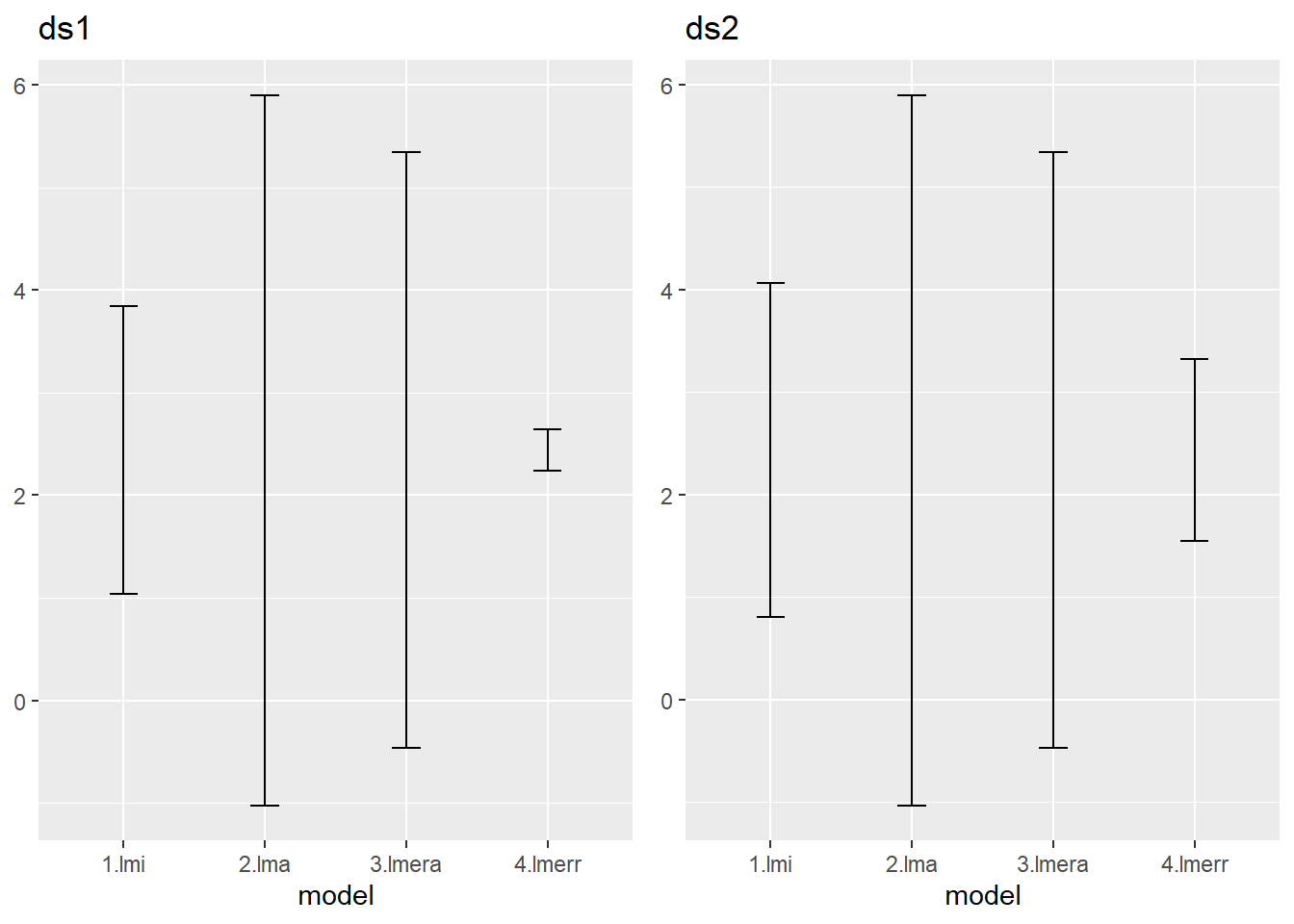
The introduction of the grouping variable rep has a huge impact on the estimate of the fixed effect. How could this be explained?
Compare with the situation where you would apply a paired t-test.
4.3 Fine tuning via bootstrapping
It was explained how confidence intervals can be estimated through bootstrapping with the advantage it is more general applicable than just the already present coefficients but also to any other combination of coefficients or predictions.
One more advantage of bootstrapping is that we can control which variance components are considered and which not in the prediction.
See the code below to understand what the argument re.form adds to predict.
mynewdata <- ds1 %>% select(treatment,rep) %>% distinct()
preds1 <- predict(lmerr.ds1,newdata=mynewdata,re.form = NA)
preds2 <- predict(lmerr.ds1,newdata=mynewdata,re.form = ~(1|rep))
preds3 <- predict(lmerr.ds1,newdata=mynewdata,re.form = NULL)
mynewdata %>% mutate(preds1=preds1,preds2=preds2,preds3=preds3)
# A tibble: 10 × 5
treatment rep preds1 preds2 preds3
<chr> <int> <dbl> <dbl> <dbl>
1 A 1 25.1 24.8 24.8
2 B 1 27.6 27.3 27.3
3 A 2 25.1 27.5 27.5
4 B 2 27.6 29.9 29.9
5 A 3 25.1 21.4 21.4
6 B 3 27.6 23.9 23.9
7 A 4 25.1 26.8 26.8
8 B 4 27.6 29.2 29.2
9 A 5 25.1 25.1 25.1
10 B 5 27.6 27.6 27.6The choice of the switches is a bit unfortunate: NA indicates not to add random effect (so only fixed effects). NULL means to include all random effects as in the model. Or you can specify the random effects you wish. the two latter are equivalent because there is only one random effect in the model.
When adding the random effect in the predict that you use in the bootstrap function, the confidence interval will be affected by this. How will become clear in the example below.
We could do this via the bootstrap we saw in the previous chapter, but because this is a central concept for mixed models, this option is even included in confint.mermod() See below how the function confint.merMod is adapted via method = "boot" and the number of bootstrap samples to take. The part of interest here (and therefore is applied here in two forms) is provided by the argument re.form.
re.form can be take the same values as explained above.
Hence let add some more versions to our confidence intervals, no with or without the random effect included in the predictions.
For ds1
cibs.ds1 <- bind_rows(
  data.frame(model="3NA.lmera",
             confint(lmera.ds1,parm = "treatmentB",
                     method="boot",nsim = 3000, re.form=NA)),
  data.frame(model="3rani.lmera",
             confint(lmera.ds1,parm = "treatmentB",
                     method="boot",nsim = 3000, re.form=~(1|animal))),
  data.frame(model="4NA.lmerr",
             confint(lmerr.ds1,parm = "treatmentB",
                     method="boot",nsim = 3000, re.form=NA)),
  data.frame(model="4rrep.lmerr",
             confint(lmerr.ds1,parm = "treatmentB",
                     method="boot",nsim = 3000, re.form=~(1|rep))),
) %>% rename(low = "X2.5..",up = "X97.5..")
Computing bootstrap confidence intervals ...
Computing bootstrap confidence intervals ...
Computing bootstrap confidence intervals ...
Computing bootstrap confidence intervals ...ci.ds1 <- bind_rows(ci.ds1,cibs.ds1)and for ds2.
cibs.ds2 <- bind_rows(
  data.frame(model="3NA.lmera",
             confint(lmera.ds2,parm = "treatmentB",
                     method="boot",nsim = 3000, re.form=NA)),
  data.frame(model="3rani.lmera",
             confint(lmera.ds2,parm = "treatmentB",
                     method="boot",nsim = 3000, re.form=~(1|animal))),
  data.frame(model="4NA.lmerr",
             confint(lmerr.ds2,parm = "treatmentB",
                     method="boot",nsim = 3000, re.form=NA)),
  data.frame(model="4rrep.lmerr",
             confint(lmerr.ds2,parm = "treatmentB",
                     method="boot",nsim = 3000, re.form=~(1|rep))),
) %>% rename(low = "X2.5..",up = "X97.5..")
Computing bootstrap confidence intervals ...
5 message(s): boundary (singular) fit: see help('isSingular')Computing bootstrap confidence intervals ...
Computing bootstrap confidence intervals ...
7 message(s): boundary (singular) fit: see help('isSingular')
1 warning(s): Model failed to converge with max|grad| = 0.00222101 (tol = 0.002, component 1)
Computing bootstrap confidence intervals ...
1 warning(s): Model failed to converge with max|grad| = 0.00855782 (tol = 0.002, component 1)ci.ds2 <- bind_rows(ci.ds2,cibs.ds2)Plot those intervals:
ci.ds1 %>% ggplot() + geom_errorbar(aes(x=model,ymin=low,ymax=up),width=.2) +
  ggtitle("ds1")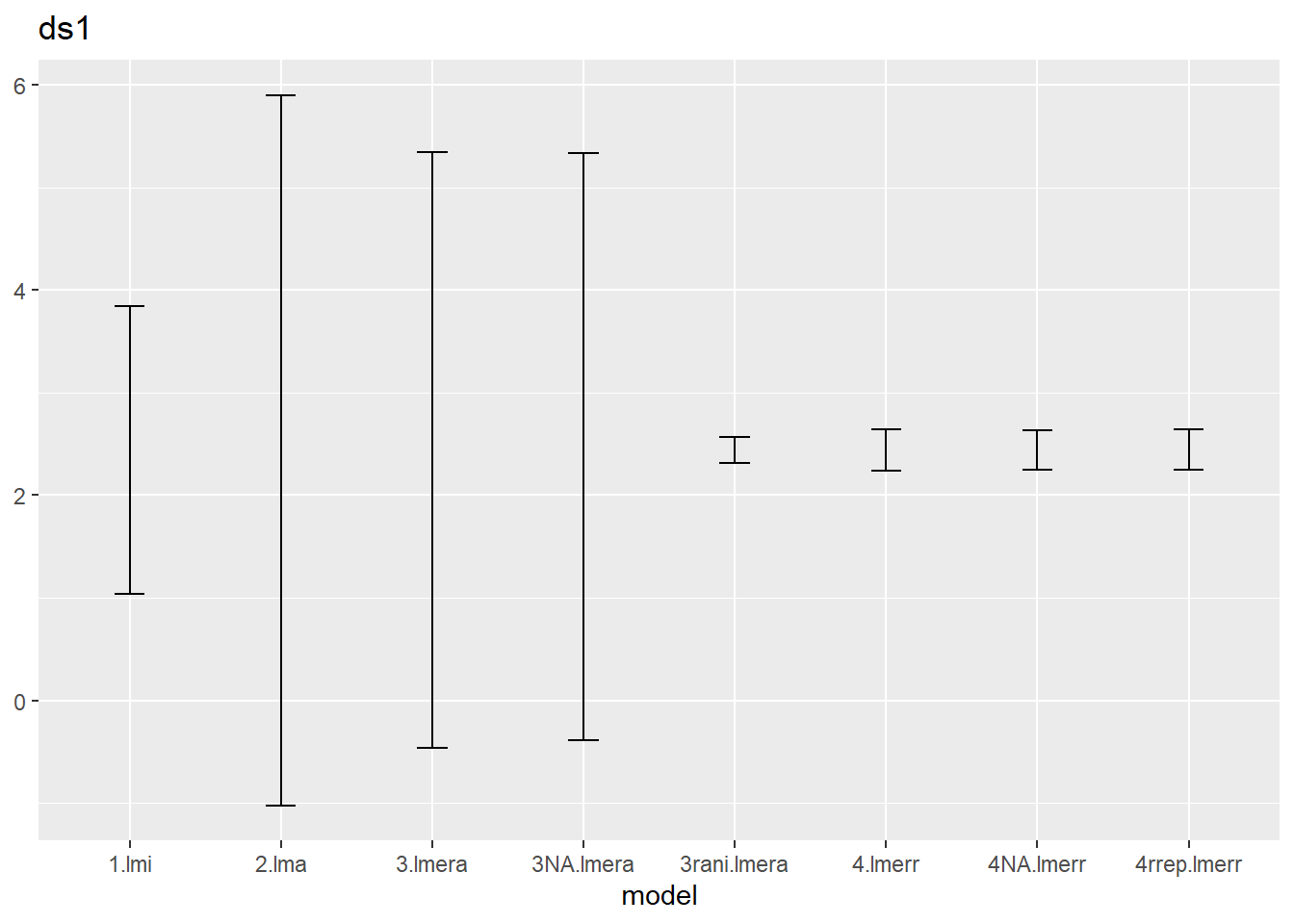
ci.ds2 %>% ggplot() + geom_errorbar(aes(x=model,ymin=low,ymax=up),width=.2) +
  ggtitle("ds2")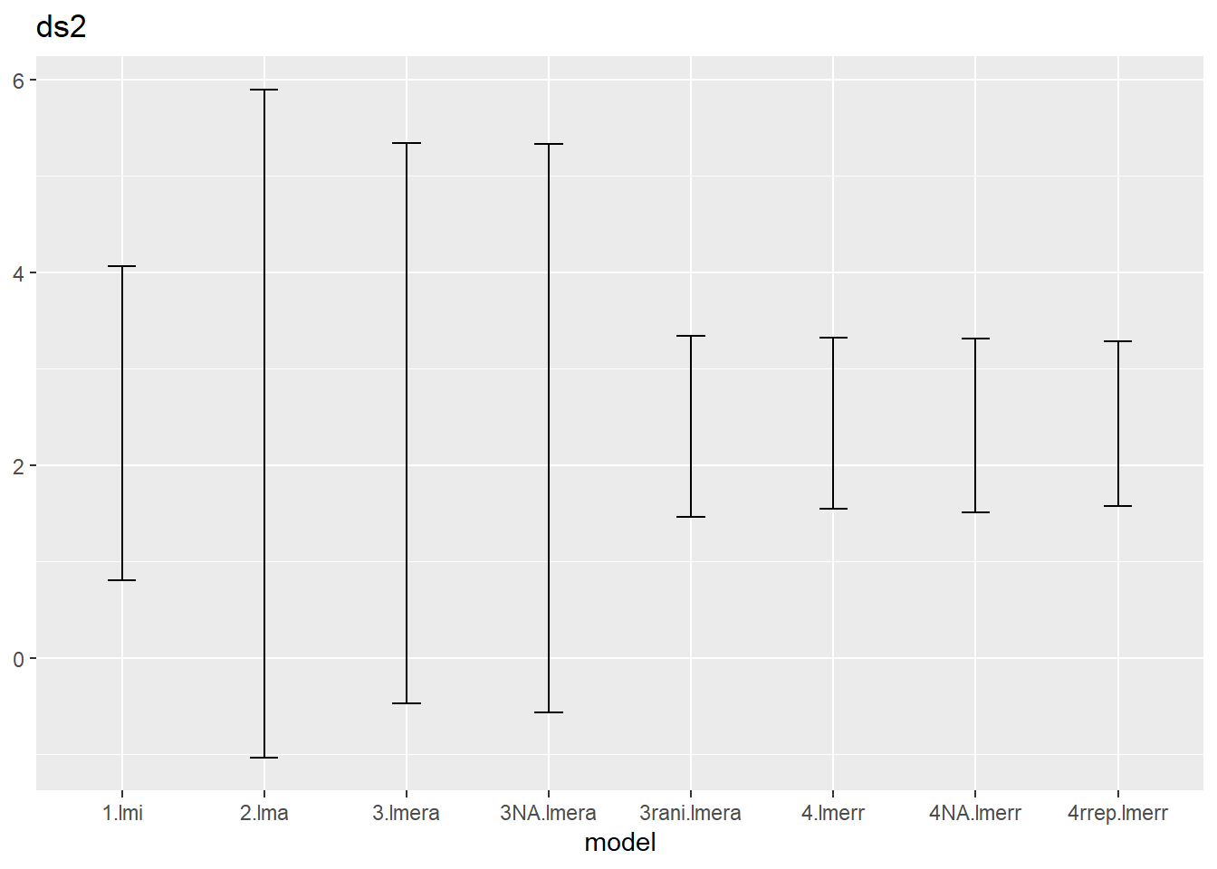
We notice that
- the default confint method (called profiling) correspond to the
re.form=NAversion of the bootstrapping, which is also the default setting ofconfint(method="boot"), - the lmera models react to this new method, but the lmerr models hardly change,
- the rani version (i.e. with random effect) for lmera is much narrower than the NA version.
Can you explain bullet 2 and 3?