# to install lme4GS:
#devtools::install_git('https://github.com/perpdgo/lme4GS/',subdir='pkg_src/lme4GS')

library(lme4GS)
data(wheat,package="BGLR")

wheat.A %>% as.vector() %>% hist(breaks=50)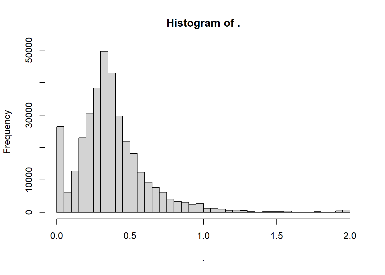
The longitudinal model of the previous section uses pre-constructed correlations between observations that are close to each other in time in the fitting process.
A similar idea is used in modelling observations that have some inherent relationship on a continuous scale. A base structure of the variance-covariance matrix is created, and is then integrated in the fitting process (see ?sec-matc). There will be only one variance component to be estimated that is the scaling factor of the provided variance-covariance matrix structure.
Suppose the constructed distance matrix \(G\) looks like this:
\[G = \begin{bmatrix} 1 & d_a & d_b & d_c & . & . & . & . \\ d_a & 1 & d_g & d_h & . & . & . & . \\ d_b & d_g & 1 & d_k & . & . & . & .\\ d_c & d_h & d_k & 1 & . & . & . & .\\ . & . & . & . & 1 & . & . & .\\ . & . & . & . & . & 1 & . & .\\ . & . & . & . & . & . & 1 & .\\ . & . & . & . & . & . & . &1\\\end{bmatrix}\]
with \(d_a\) the (inverse) distance or relatedness between object 1 and 2, \(d_b\) between object 1 and object 3, and so on. With the \(d\)s between 0 and 1, with 1 being identical (no distance).
Remember that the classic grouped mixed model or single level hierarchical model can be represented like this:
\[Y = X\beta + Zu + \varepsilon\] with X and Z are 0-1 incidence matrices (also called design matrices, respectively for fixed and random effects), \(\beta\) are the to-be-estimated fixed effects coefficients, and \(u\) the random effects following a multivariate normal \(MVN(0,\sigma_u^2V)\), and \(\varepsilon\) the residuals following a normal distribution \(N(0,\sigma^2)\).
Whereas the variance-covariance matrix \(V\) in the grouped model is created for us via the software depending on which random effects we asked, is will now be of the form \(\sigma_r^2G\). Hence only variance component \(\sigma_r\) needs to be estimated.
A common use case is where the \(G\) matrix represents a relatedness matrix, where the genetic proximity, as defined by a pedigree or by calculation a distance matrix on the basis of genotype data. Yet the relatedness could be anything else (a physical distance, a similarity matrix between locations based on a multivariate environmental parameters,…)
To illustrate this principle we use the package lme4GS which is an extension of lme4.
The example is a breeding trial on a few hundred less or more related wheat lines. The data are obtained from the the package BGLR. The wheat data therein have a wheat.A matrix, which is a square symmetric matrix with in rows and columns the tested wheat lines, and carrying numbers between 0 (no relationship) and 2 (100% clones).
# to install lme4GS:
#devtools::install_git('https://github.com/perpdgo/lme4GS/',subdir='pkg_src/lme4GS')
library(lme4GS)
data(wheat,package="BGLR")
wheat.A %>% as.vector() %>% hist(breaks=50)
The matrix wheat.Y contains the yields measured in a number of trials for each of the wheta lines. It requires some reformatting into a long data frame to allow it being processed by lme4GS.
wheat.Y.ldf <- wheat.Y %>%
  as_tibble(rownames="genotype") %>%
  rename_with(.fn=function(x) paste0("trial",x),.cols=(-genotype)) %>%
  pivot_longer(cols=starts_with("trial"),values_to="yield",names_to="trial")
The model without G (wheat.m1) and with G (wheat.m2) are fitted. In both cases genotype is a random effect, but in the latter extra refinement about the connection is provided.
wheat.m1 <- lme4::lmer(
  data = wheat.Y.ldf,
  yield ~ trial + (1|genotype)
)

wheat.m2 <- lme4GS::lmerUvcov(
  data = wheat.Y.ldf,
  yield ~ trial + (1|genotype),
  Uvcov=list(genotype=list(K=wheat.A))
)
Factoring method for matrix K associated with genotype was set to 'auto'Computing relfac using Choleskyiteration: 1
x = 0.800380
f(x) = 6713.109459
iteration: 2
x = 1.400666
f(x) = 7002.570832
iteration: 3
x = 0.200095
f(x) = 6628.125507
iteration: 4
x = 0.250750
f(x) = 6606.972653
iteration: 5
x = 0.400821
f(x) = 6588.152572
iteration: 6
x = 0.404444
f(x) = 6588.366062
iteration: 7
x = 0.394818
f(x) = 6587.858105
iteration: 8
x = 0.388816
f(x) = 6587.638853
iteration: 9
x = 0.376810
f(x) = 6587.432137
iteration: 10
x = 0.374696
f(x) = 6587.428453
iteration: 11
x = 0.374096
f(x) = 6587.429222
iteration: 12
x = 0.374971
f(x) = 6587.428370
iteration: 13
x = 0.375031
f(x) = 6587.428374
iteration: 14
x = 0.374911
f(x) = 6587.428374
iteration: 15
x = 0.374970
f(x) = 6587.428370The random part of the summary output:
summary(wheat.m1)$varcor Groups Name Std.Dev.
genotype (Intercept) 0.43277
Residual 0.90150 summary(wheat.m2)$varcor Groups Name Std.Dev.
genotype (Intercept) 0.33658
Residual 0.89762 The genotype variance component is smaller in the second model but has a different meaning.
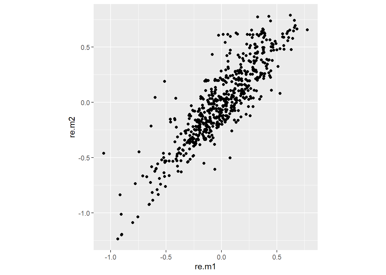
The biggest impact can be seen on the blups of the wheat lines in both models. (remark: due to a different parameterisation, the fixed intercept of wheat.m2 needs to be added to the blups of wheat.m2 )
KK <- data.frame(genotype=rownames(wheat.Y),
  re.m1=ranef(wheat.m1)$genotype[,1],
  re.m2=ranef(wheat.m2)$genotype[,1] + summary(wheat.m2)$coefficients[1,"Estimate"]
  )

KK %>% head()
genotype re.m1 re.m2
1 775 -0.6508369 -0.92288952
2 2166 0.2957093 0.35323191
3 2167 -0.9058979 -1.01421808
4 2465 0.5635522 0.58873260
5 3881 -0.1876134 0.05038266
6 3889 0.3835646 0.45027283ggplot(KK,aes(y=re.m2,x=re.m1)) +
geom_point() +
coord_fixed()