model <- linearModelFunction(data = ...,
                             formula = y ~ 'fixed effects' + ('random effects'),
family = ..., extra model-specific arguments)1 How-to in R
Several algorithms have been developed to solve the linear model. Some are fast and good enough for simple models (LM: balanced data sets, no random effects, normally distributed residuals). Others are necessarily more complex for the more complex models (GLM, LMM and GLMM: complex data sets, non-normal and/or non-independent residuals).
Because of the importance and diversity of the linear model several methods to solve linear models are implemented in R. These methods use often very different algorithms. Luckily there is some consistency in the interface and output that is used in the various packages and approaches.
The general syntax for running these models in R is
and bring the most important output together by
summary(model).
Other useful functions like predict, plot, residuals, sigma can be used across the various packages and functions.
The y in the left hand side of the formula is obviously the response, the part that needs to be modelled. This can be complex in its own. In this course we will consider only simple univariate variables, but not necessarily normal or even continuous.
For very simple situation the ordinary least squares may be sufficient, which is implemented in lm (R package stats). For non-normal responses maximum likelihood-based glm (R package stats) can be used. However, rapidly experiments become more complex and have non-independent observations or random effects. Mixed models based on maximum likelihood need to be used (gls, lme from R package nlme or lmer and glmer from R package lme4). Additive models are linear models with the capability of fitting smooth functions (see mgcv or gamm4) and require also more complex algorithms.
Linear models are not only popular in frequentist statistic but also in Bayesian statistics. The R package brms is based on Stan and does full Bayesian inference, but uses the standard R linear models conventions. It is therefore an easy transition to Bayesian statistics. Besides the Bayesian context, another advantage is that the algorithms used to solve the linear models, are very flexible and can handle situations that other algorithms cannot properly deal with.
2 Chicken feed
This will all become clear when running actual linear models in R on a data set about raising young chicks. You can download the data set here. It is stored as an R object.
Broiler chicken production from one-day chick to slaughter occurs in 8 weeks. From day 1 to day 21 the chickens are raised on a starter diet and are then switched to a grower diet.
The feed mix requires minerals. A chicken feed producer tested alternative sources of minerals. The experiment used 20 cages, with 4 chickens each.
The data are stored in the data frame chickensC. The sources of the minerals is contained in the variable supplier. The original source is called Our104. For the time being the response variable is endweight, which is the weight of each chicken before slaughter. For each chicken the cage in which it is raised is provided in the variable cage. There were 4 chickens in each cage.
load("data/chickensC.obj")
head(chickensC,10)
chicken cage supplier startweight endweight
1 chick1 cage1 AV102 744.4 1803.2
2 chick2 cage1 AV102 747.7 1835.5
3 chick3 cage1 AV102 765.6 1838.3
4 chick4 cage1 AV102 750.7 1820.4
5 chick5 cage2 BK77 751.3 1788.5
6 chick6 cage2 BK77 767.2 1831.6
7 chick7 cage2 BK77 754.6 1796.8
8 chick8 cage2 BK77 737.3 1753.1
9 chick9 cage3 CM10 743.1 1811.2
10 chick10 cage3 CM10 745.5 1852.6Plotting the data is the best way to get a good overview of experimental structure and the response. In the plot below the 5 sources are compared. Each dot is a chicken. The colour and position of the dots indicates which chickens are raised together. Some sources are clearly worse than Our104, while others seems to be equivalent.
ggplot(data=chickensC,
  aes(y=endweight,x=supplier,color=cage,group=cage)) +
  geom_point(size=2, alpha=0.7,position=position_dodge(width=0.3)) +
  theme_bw() +
  theme(panel.grid.major.x = element_blank(),legend.position = "none")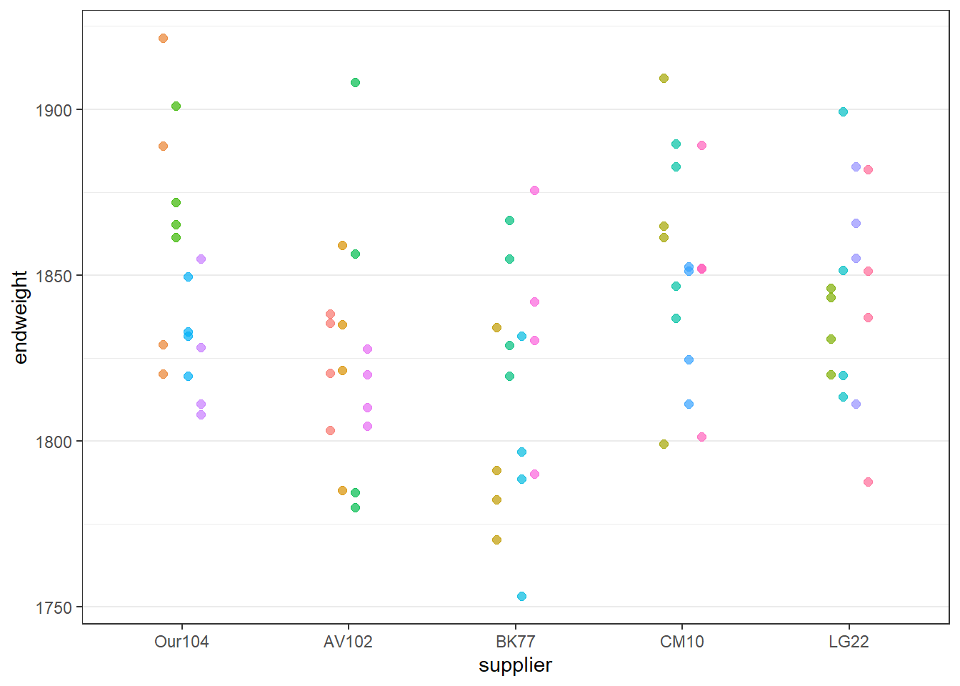
3 Modelling
3.1 A basic linear model
We can fit a linear model to these data. We start with the function lm(). The use of the function is the standard lm(data = …, y ~ factor) statement.
With the function summary() the model is summarized and possibly intersting output printed.
modlm.1.0 <- lm(data=chickensC,
                endweight~supplier)

summary(modlm.1.0)
Call:
lm(formula = endweight ~ supplier, data = chickensC)

Residuals:
    Min      1Q  Median      3Q     Max
-62.850 -24.011   0.125  16.300  83.706

Coefficients:
              Estimate Std. Error t value Pr(>|t|)
(Intercept)   1849.631      8.164 226.563  < 2e-16 ***
supplierAV102  -25.338     11.545  -2.195  0.03129 *
supplierBK77   -33.681     11.545  -2.917  0.00466 **
supplierCM10     1.888     11.545   0.163  0.87058
supplierLG22    -6.100     11.545  -0.528  0.59882
---
Signif. codes:  0 '***' 0.001 '**' 0.01 '*' 0.05 '.' 0.1 ' ' 1

Residual standard error: 32.66 on 75 degrees of freedom
Multiple R-squared:  0.1691,    Adjusted R-squared:  0.1248
F-statistic: 3.817 on 4 and 75 DF,  p-value: 0.007051
The output repeats the call, then gives some difficult to interpret information about the residuals, and ends with a table with the coefficients and some statistics.
Of interest for now is the central table with the coefficients. These are the coefficients or
Of interest for now is the central table with the coefficients. These are the coefficients or \(\beta\)’s for the dummy variables we discussed in box 1, each taking the presence or absence of a particular supplier. There are only 4 suppliers named explicitly. This is because AV102 is used as a reference and serves as intercept for the linear model. The other suppliers are estimated as how they differ from the reference. The estimate for AV102 is about 1850 g and matches our expectations based on the plot. BK77 yields 25 g less than AV102. Alternative choices for the coding are possible, but this one is convenient for making comparisons (or contrasts) between treatments.
The standard errors on these estimates are all the same except again the one for the intercept, which is smaller. This is logic as for the intercept only the uncertainty of AV102 matters, while for the estimates of the differences both the uncertainty of the supplier and that of AV102 are involved. You could have obtained this yourself via:
s <- sigma(modlm.1.0)
s
[1] 32.65547# intercept:
sqrt(s^2/16)[1] 8.163867# estimates of the differences:
sqrt(2*s^2/16)[1] 11.54545The rest of the table (t and P values) are straightforward to derive as well. The P-value for the intercept is of no interest (obviously the chickens have some weight that is non-zero), while the P-value of the differences directly give a measure for the statistical significance of the difference between two suppliers.
However, the above analysis is wrong. When looking at the plot of the raw data, we realize that the chickens raised in the same cage are more alike when compared to a chicken from another cage. The observations are not independent. One way to solve this problem is by using cage as our observational unit in the model. Therefore, we first average the weights obtained in each case.
chickensC.s <- chickensC %>% group_by(cage,supplier) %>%
  summarise(endweight=mean(endweight),.groups="drop")

modlm.s.1.0 <- lm(data=chickensC.s,
                  endweight~supplier)

summary(modlm.s.1.0)
Call:
lm(formula = endweight ~ supplier, data = chickensC.s)

Residuals:
     Min       1Q   Median       3Q      Max
-24.1313 -10.6156   0.4188  10.6781  26.4500

Coefficients:
              Estimate Std. Error t value Pr(>|t|)
(Intercept)   1849.631      8.745 211.502   <2e-16 ***
supplierAV102  -25.338     12.368  -2.049   0.0584 .
supplierBK77   -33.681     12.368  -2.723   0.0157 *
supplierCM10     1.887     12.368   0.153   0.8807
supplierLG22    -6.100     12.368  -0.493   0.6290
---
Signif. codes:  0 '***' 0.001 '**' 0.01 '*' 0.05 '.' 0.1 ' ' 1

Residual standard error: 17.49 on 15 degrees of freedom
Multiple R-squared:  0.4701,    Adjusted R-squared:  0.3287
F-statistic: 3.326 on 4 and 15 DF,  p-value: 0.03867
The averaging has no impact on the estimates (in this balanced data set), but the standard errors increase, what obviously impacts the t-values and p-values.
3.2 A more appropriate mixed linear model
There are more elegant ways to deal with dependencies. We already explained that non-independence of observations can be tackled via random effects. Models with fixed and random effects are called mixed models. The function lmer() of package lme4 can be used for this.
The model is run on the original data (chicken-level). An extra component (the random effect) is added to indicate that chickens should be grouped by cage.
library(lme4)Loading required package: Matrix
Attaching package: 'Matrix'The following objects are masked from 'package:tidyr':
expand, pack, unpackmodlmer.1.0 <- lmer(data=chickensC,
endweight ~ supplier + (1|cage))
summary(modlmer.1.0,correlation=FALSE)Linear mixed model fit by REML ['lmerMod']
Formula: endweight ~ supplier + (1 | cage)
Data: chickensC
REML criterion at convergence: 749.4
Scaled residuals:
Min 1Q Median 3Q Max
-1.8436 -0.7247 0.0341 0.5756 2.5723
Random effects:
Groups Name Variance Std.Dev.
cage (Intercept) 49.15 7.011
Residual 1027.06 32.048
Number of obs: 80, groups: cage, 20
Fixed effects:
Estimate Std. Error t value
(Intercept) 1849.631 8.745 211.502
supplierAV102 -25.338 12.368 -2.049
supplierBK77 -33.681 12.368 -2.723
supplierCM10 1.887 12.368 0.153
supplierLG22 -6.100 12.368 -0.493The output is nearly identical to the simple model on the cage averages. Estimates and standard errors of the fixed effects of this model and of the coefficients on the cage-level model are identical.
There are no p-values in this output. If you really need them you can use in this simple case the function lmer() from the package lmerTest. It works the same, but the output via summary() will be slightly different and will contain p-values.
We get an extra part on the the random effect. The residual level standard deviation is similar to the residual error in the simple model on chicken-level. New is the effect on cage-level, which indicates how strong the cages vary among each other. This splits up the variance components, a feature that will come in handy when designing more complex experiments.
Besides this split in variance components, the model on cage-level via prior averaging does an as a good job as this mixed model. So why do we need the more complex mixed model? Simply because the trick with the averaging only works with nice and neat experiments where all treatments have an equal number of observations. We all know that this only happens in theoretical statistics courses. In reality, experiments are more messy, either by design or because of bad luck.
3.3 Assumption checking
Linear models will only deliver reliable output if certain assumptions are met. It would lead us too far in this stage to go into details on this subject, since the various different models make different assumptions. Certain variants of the linear model are purposefully developed to overcome problems with these assumptions that can not be dealt with by basic linear models.
Most common (and useful) diagnostics of the validity of the models are graphical checks of the residuals (distribution, independence, variation in function of the fit). R models can usually be checked by the generic function plot that provides graphs of interesting views on the residuals for the specific model at hand. If you are in the dark on this subject, read more about it.
3.4 On the side:
3.4.1 Multiple testing
For completeness we also mention the issue of multiple testing. This is the problem that if several hypothesis tests (comparison of several mineral mixes) are performed simultaneous, classic statistical tests become too optimistic. The probability that you find a significant result purely by chance is not the set \(\alpha\) (e.g. 5%) but a multiple of this \(\alpha\).
We will not elaborate on this issue here and what the solutions are. Also on this subject you will have to read elsewhere.
3.4.2 Recode the factor to a more helpful form
We have seen that one source of the minerals is taken as reference. The others are compared to it. The research question is about comparison with a specific mineral supply, the original standard source Our104. By default the levels are ordered alphabetically and the first one (AV102) becomes the reference. It makes things simpler to utilise the standard as reference. All the coefficients of the model get an easily interpretable meaning in that way.
Making Our104 the reference can be done by re-levelling the factor supplier.
chickensC$supplier <- relevel(chickensC$supplier,ref="Our104")

modlmer.1.0 <- lmer(data=chickensC,
                    endweight~supplier + (1|cage))

summary(modlmer.1.0,correlation=FALSE)
Linear mixed model fit by REML ['lmerMod']
Formula: endweight ~ supplier + (1 | cage)
Data: chickensC
REML criterion at convergence: 749.4
Scaled residuals:
Min 1Q Median 3Q Max
-1.8436 -0.7247 0.0341 0.5756 2.5723
Random effects:
Groups Name Variance Std.Dev.
cage (Intercept) 49.15 7.011
Residual 1027.06 32.048
Number of obs: 80, groups: cage, 20
Fixed effects:
Estimate Std. Error t value
(Intercept) 1849.631 8.745 211.502
supplierAV102 -25.338 12.368 -2.049
supplierBK77 -33.681 12.368 -2.723
supplierCM10 1.887 12.368 0.153
supplierLG22 -6.100 12.368 -0.493