We have been focussing on grouping in the observation. Other types of dependencies can exist within data sets. A very common one is several observations over time on the same subject.
The chicken data contain 4 time points at which the chickens have been weighted. It requires a bit or reorganization to visualize the change in weight over time. Luckily it is the same reorganization that will be needed to fit longitudinal models.
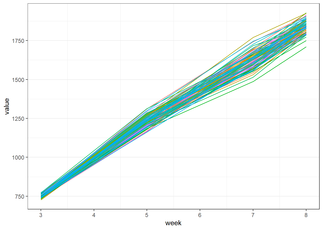
chickensL <- chickens %>%pivot_longer(cols=c(startweight,week5,week7,endweight),names_to ="time") %>%mutate(week =case_when(time =="startweight"~3, time =="week5"~5, time =="week7"~7, time =="endweight"~8,TRUE~0)) chickensL$supplier <-relevel(chickensL$supplier,ref="Our104")chickensL %>%ggplot(aes(y=value,x=week,color=cage,group=chicken)) +geom_line() +theme_bw() +theme(panel.grid.major.x =element_blank(),legend.position ="none")
The graph shows a steady increase in weight of the chickens. Depending on what the purpose is of the repeated measurements, we could opt for different models.
We could consider the repeated measurements as a mean to improve the accuracy by having more measurements. Time could be a random factor in that situation, similar to the models we have seen in previous chapters.
Another reason could be to compare the growth rates obtained with the various feeds. In that case time can be added as factor in other to obtain a random slope, in addition to a random intercept for each chicken. These models are called random slope models. In lmer it is indicated via (1+week|chicken).
Linear mixed model fit by REML ['lmerMod']
Formula: value ~ supplier + (1 | cage) + (1 + week | chicken)
   Data: chickensL
Control: lmerControl(optimizer = "Nelder_Mead")

REML criterion at convergence: 4088.2

Scaled residuals:
    Min      1Q  Median      3Q     Max
-1.8174 -0.5739 -0.1146  0.5086  2.7879

Random effects:
 Groups   Name        Variance Std.Dev. Corr
 chicken  (Intercept) 796267   892.34
          week         46420   215.45   -1.00
 cage     (Intercept)      0     0.00
 Residual               1293    35.95
Number of obs: 352, groups:  chicken, 88; cage, 22

Fixed effects:
              Estimate Std. Error t value
(Intercept)   1014.443      4.785 212.011
supplierAV102    9.198      7.566   1.216
supplierBK77    -6.071      7.566  -0.803
supplierCM10    11.929      7.566   1.577
supplierLG22     2.873      7.566   0.380
optimizer (Nelder_Mead) convergence code: 0 (OK)
boundary (singular) fit: see help('isSingular')
In the output, the random effects reflects the grouping: a classic grouping effect (intercept only) for cage and a regression (with intercept and slope) for chicken. The cage is so small it got absorbed elsewhere.
The fixed effect provides the level of the reference feed and the deviations caused by the various feeds. The reference level is reflecting the weight at some intermediate time point (the average of 3, 5, 7 and 8 weeks).
An alternative model is by considering time as a fixed effect as well. The observations of a particular chicken are reasonably linear, hence a linear regression model for the fixed effects makes sense. The random slope model will allow by-chicken random deviations from the main fixed slope (one for each supplier). The cage random effect will still be included.
Linear mixed model fit by REML ['lmerMod']
Formula: value ~ supplier * week + (1 | cage) + (1 + week | chicken)
   Data: chickensL
Control: lmerControl(optimizer = "Nelder_Mead")

REML criterion at convergence: 3519.9

Scaled residuals:
    Min      1Q  Median      3Q     Max
-2.1932 -0.6454 -0.2135  0.5436  2.7803

Random effects:
 Groups   Name        Variance  Std.Dev.  Corr
 chicken  (Intercept) 1.521e+02 1.233e+01
          week        3.336e+01 5.775e+00 -1.00
 cage     (Intercept) 2.635e-07 5.133e-04
 Residual             1.152e+03 3.394e+01
Number of obs: 352, groups:  chicken, 88; cage, 22

Fixed effects:
                   Estimate Std. Error t value
(Intercept)        110.3844    11.2224   9.836
supplierAV102       22.9179    17.7441   1.292
supplierBK77        32.1231    17.7441   1.810
supplierCM10        18.8303    17.7441   1.061
supplierLG22         4.9343    17.7441   0.278
week               218.1237     2.1551 101.214
supplierAV102:week  -3.3103     3.4075  -0.971
supplierBK77:week   -9.2153     3.4075  -2.704
supplierCM10:week   -1.6651     3.4075  -0.489
supplierLG22:week   -0.4974     3.4075  -0.146
optimizer (Nelder_Mead) convergence code: 0 (OK)
boundary (singular) fit: see help('isSingular')
In the fixed effects part we now get also a slope by supplier. BK77 starts high but has a slower gain in the course of the experiment. The random effect for week is much lower, because majority of the variability is absorbed by the fixed effect.
Remark that the intercept has changed. It now is an actual intercept and reflects the weight at time zero. This is not so interesting information. Therefore it is usually more informative to rescale the time and set 0 where it provides useful information. For instance, have the intercept at time point week = 5, would make it comparable to the previous model. Any interesting time point can be chosen for this purpose.
We could think about another model where the deviation from the slope is linked to the cage rather than to the chicken, but apparently the extra parameter fitted by modlmer.L3 is justified as shown by anova() of the competing models.
6.2 Predictions and bootstraps of more complex questions
The model output becomes more complex, and usually what we actually need can not be found directly in the default model output. The current output is about weights at week 0 (not clear what this actually means…) and a slope. Suppose that chickens are normally slaughtered after 7 and a half weeks. Predictions of the weights at that time would be handy.
A new dataset with same names as the original data set but with the new levels of interest is created and provide to the predict() function.
If we apply this in combination with a bootstrap, we obtain confidence intervals on these predictions.
# prediction + bootstraps can be used to find confidence intervalsnd <-data.frame(supplier =levels(chickensL$supplier),week=7.5)bootfun <-function(mod){predict(mod,newdata=nd,re.form =NA)}bs <-bootMer(modlmer.L3,bootfun,nsim=500)str(bs$t)
Starting from the bootstrapped estimates, other contrasts or derived values can be calculated. For instance but for the difference with the reference (i.e. the first element of the extraction).
Hence the output is similar as what we obtained by shifting the intercept (modlmer.L3_shifted). The advantage of doing it this way is it general applicability. This is an illustration of a more general way of extracting some complex contrast (or proportion for instance) from mixed models.
6.3 More complex dependencies in time
Obviously the previous approach is only practical when there is some simple relationship that can be modelled in the fixed effect and/or a slope.
In the situation where there is no linear relationship other options are available.
One option is to model the time as an autoregressed effect: models with a correlation between an observation and the previous observation on the same subject. All subjects can evolve independently along its own pattern. They are typically fitted with the packages nlme or brms. The latter we will explain later in this chapter.
When the observations follow a pattern, particularly when that pattern has common features among the subjects, generalized additive models can be used. These models have also mixed variants. See package gamm4. This we will not treat in this course.
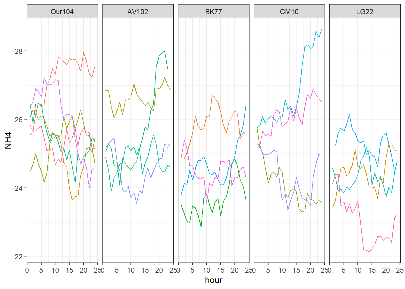
The chicken experiment also measured ammonia release from the cages. During an entire day, at every hour, air samples haven taken and analysed for ammonia. The results are in a separate data set (get it here) and is plotted below.
From the graph it is clear that the observations are not independent (an observation resembles the one from an hour before). We need models that acknowledge correlations between adjacent observations, but we cannot use the simple linear relationship with time.
Here we get in another type of mixed models where observations are not (only) grouped but have a continuous tight or less tight relationship.
We will use brms to illustrate this. And fir three models: one that ignores all dependencies (the classic fixed model), a model that considered only the grouping effect of cages, and a third one that additionally models observations from a same cage with a autoregressive or AR connection among them, meaning that observations are correlated to the observations that happened before (on the same subject). In this case, we ask for just for AR1, that is only the previous observation is considered (ar(..., p=1). We could ask for more (p = 2 or 3). An additional parameter \(\phi\) is entered in the model. It models the dependency as \(\phi^1, \phi^2, ...\) with the exponent being the order of separation in the time series. When \(\phi\) is smaller than 1 this gives an ever further decreasing correlation.
We compare three models: one assuming total independence, one assuming grouping by cage, and finally one that assumes grouping by cage and an AR1 between consecutive measurements.
The last two models have a random group effect cage.
The code in the chunks below extracts the blups for the cages (the part ranef()).
The rest of the code is not meant to provide directly interpretable output, but is used her solely to show that there is even more shrinking in the model with an autoregression component mar.3.brms which leads to stabilization. Which illustrates that modelling the dependence helps.