load("data/chickens.obj")
chickens$supplier <- relevel(chickens$supplier,ref="Our104")3 Adding complexity
3.1 Unequal replication
Suppose that the experiment used 22 cages and that the chickens in the extra cage 21 were fed with CM10 and those in cage 22 with BK77. The data set chickens contains those 22 cages. You can download it here
modlmer.1.1 <- lmer(data=chickens,
                    endweight~supplier + (1|cage))

summary(modlmer.1.1,correlation=FALSE)
Linear mixed model fit by REML ['lmerMod']
Formula: endweight ~ supplier + (1 | cage)
Data: chickens
REML criterion at convergence: 845.6
Scaled residuals:
Min 1Q Median 3Q Max
-2.16198 -0.62601 -0.03249 0.63994 2.13993
Random effects:
Groups Name Variance Std.Dev.
cage (Intercept) 383.8 19.59
Residual 1095.6 33.10
Number of obs: 88, groups: cage, 22
Fixed effects:
Estimate Std. Error t value
(Intercept) 1851.521 10.470 176.847
supplierAV102 -9.958 16.554 -0.602
supplierBK77 -45.302 16.554 -2.737
supplierCM10 1.548 16.554 0.094
supplierLG22 -5.521 16.554 -0.334So, unequal replication does not create trouble. On the contrary, we have extra observations what normally leads to more accurate estimates.
Only the estimates of the two suppliers with the extra cage have changed. Yet, all standard errors have changed, including the one for the intercept.
This raises questions on experimental design:
- Is the conclusion about a treatment affected by other treatments in the experiment?
- Can we optimise the choice of what to put in the extra cages?
What do you think?
3.2 More than one random effect
The idea of the random effect can be expanded to several random effects.
Suppose that the chicken experiment happened not in one run but in several runs, or that the cages were placed in several, supposedly identical rooms. In that case an additional random needs to be added.
Data set chickens contains an additional factor room.
table(chickens$room,chickens$cage)
        cage1 cage10 cage11 cage12 cage13 cage14 cage15 cage16 cage17 cage18
  room1     4      0      0      0      0      0      0      0      0      0
  room2     0      0      0      0      0      0      0      0      0      0
  room3     0      0      0      0      0      0      0      0      0      0
  room4     0      4      4      4      0      0      0      0      0      0
  room5     0      0      0      0      4      4      4      0      0      0
  room6     0      0      0      0      0      0      0      4      4      4
  room7     0      0      0      0      0      0      0      0      0      0

        cage19 cage2 cage20 cage21 cage22 cage3 cage4 cage5 cage6 cage7 cage8
  room1      0     4      0      0      0     4     0     0     0     0     0
  room2      0     0      0      0      0     0     4     4     4     0     0
  room3      0     0      0      0      0     0     0     0     0     4     4
  room4      0     0      0      0      0     0     0     0     0     0     0
  room5      0     0      0      0      0     0     0     0     0     0     0
  room6      0     0      0      0      0     0     0     0     0     0     0
  room7      4     0      4      4      4     0     0     0     0     0     0

        cage9
  room1     0
  room2     0
  room3     4
  room4     0
  room5     0
  room6     0
room7 0ggplot(data=chickens,
aes(y=endweight,x=supplier,color=cage,group=cage)) +
geom_point(size=2, alpha=0.7,position=position_dodge(width=0.3)) +
theme_bw() +
theme(panel.grid.major.x = element_blank(),legend.position = "none") +
facet_wrap(~room)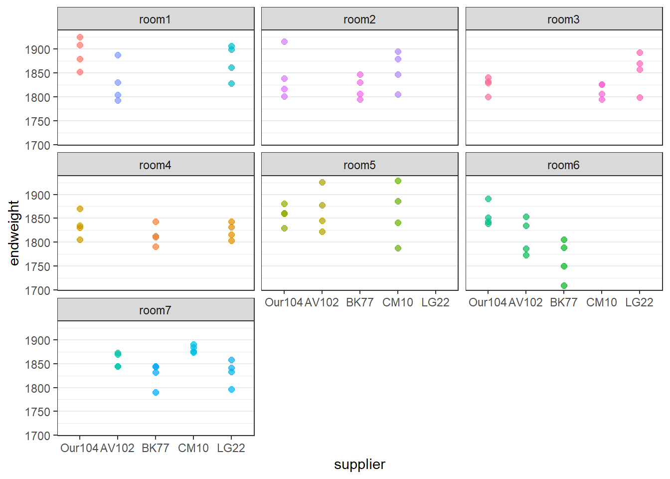
A cage cab be in only one room. So cage is nested within room. These nested random effects are indicated by (1\|room/cage) in the formula.
modlmer.1.2 <- lmer(data=chickens,
                    endweight~supplier + (1|room/cage))

summary(modlmer.1.2,correlation=FALSE)
Linear mixed model fit by REML ['lmerMod']
Formula: endweight ~ supplier + (1 | room/cage)
Data: chickens
REML criterion at convergence: 844.9
Scaled residuals:
Min 1Q Median 3Q Max
-2.17572 -0.61365 -0.04257 0.65493 2.11671
Random effects:
Groups Name Variance Std.Dev.
cage:room (Intercept) 240.7 15.52
room (Intercept) 141.0 11.87
Residual 1095.6 33.10
Number of obs: 88, groups: cage:room, 22; room, 7
Fixed effects:
Estimate Std. Error t value
(Intercept) 1852.727 10.375 178.583
supplierAV102 -14.226 15.084 -0.943
supplierBK77 -44.830 15.084 -2.972
supplierCM10 -1.273 15.084 -0.084
supplierLG22 -7.344 15.084 -0.487We can formally compare both models
anova(modlmer.1.1,modlmer.1.2)refitting model(s) with ML (instead of REML)Data: chickens
Models:
modlmer.1.1: endweight ~ supplier + (1 | cage)
modlmer.1.2: endweight ~ supplier + (1 | room/cage)
npar AIC BIC logLik deviance Chisq Df Pr(>Chisq)
modlmer.1.1 7 893.25 910.59 -439.63 879.25
modlmer.1.2 8 894.18 914.00 -439.09 878.18 1.0678 1 0.3015This test tells us that it is not justified to add the level room to the model. The more complex model does not fit the data better and hence it is not needed to spend extra parameter estimate on it. Often the AIC (The Akaiki Information Criterion) is used for this decision.
Check also the impact on the estimates.
Because cages have their own unique identifier, the lmer function can determine whether the random factors are nested or not. So in this situation the following model is equivalent to the previous.
# alternative (because cage have distinct names...)
modlmer.1.2b <- lmer(data=chickens,
                     endweight~supplier + (1|cage) + (1|room))