2  Extracting extra results from the model object

2.1 Confidence intervals

The estimates and their confidence intervals should form the basis of your communication. Plotting these conveys the message usually best.

Remark: In frequentist statistics a value of a parameter is fixed, yet unknown. The definition of a 95% confidence interval is that if you would run 100 independent experiments, at least 95 of the obtained confidence intervals are expected to include the true value of the parameter. Bayesian statistics considers a parameter as a random variable with a probability distribution. The bayesian alternative to a 95% confidence interval is called a 95 % credible interval, which is a range which includes 95% of the mass of the posterior probability distribution of the parameter. The latter is what is also what we like to assume about the confidence interval, but is not the case.

Confidence intervals based on fixed models are calculated from the standard errors on the fixed effects. We can do something similar in th case of mixed models to calculate approximate confidence intervals on the estimates of the differences.

as.data.frame(summary(modlmer.1.0)$coefficients) %>% 
  mutate(lwr=Estimate - 1.96*`Std. Error`,upr=Estimate + 1.96*`Std. Error`)
                Estimate Std. Error     t value        lwr         upr
(Intercept)   1849.63125   8.745221 211.5019558 1832.49062 1866.771882
supplierAV102  -25.33750  12.367610  -2.0486983  -49.57801   -1.096985
supplierBK77   -33.68125  12.367610  -2.7233436  -57.92176   -9.440735
supplierCM10     1.88750  12.367610   0.1526164  -22.35301   26.128015
supplierLG22    -6.10000  12.367610  -0.4932239  -30.34051   18.140515

A more correct way of calculating the confidence intervals in the case of mixed models is done via profiling of the maximum likelihoods with the function confint.

Check out the documentation for confint() and confint.merMod(). Remember that in R, if you apply confint() on a mixed model (is of class merMod), you apply in reality confint.merMod().

The intervals differ slightly.

confint(modlmer.1.0,parm="beta_")
                   2.5 %      97.5 %
(Intercept)   1833.95061 1865.311885
supplierAV102  -47.51327   -3.161733
supplierBK77   -55.85702  -11.505483
supplierCM10   -20.28827   24.063267
supplierLG22   -28.27577   16.075767

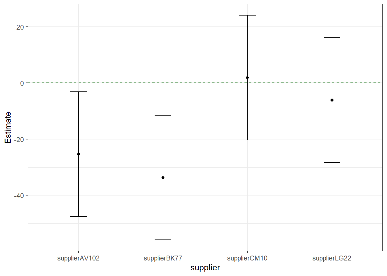
Bringing estimates and confidence intervals and plotting, should become your preferred method to interpret and to convey your conclusions.

In the plot below the estimates of the differences of the chicken weights of all alternative feeds compared to chickes fed with Our104 are provided. A line is drawn to indicate where the zero effect would be. Confidence intervals that include this line point at mineral mixes that are not significantly different from Our104.

results.1.0 <- cbind(
  as.data.frame(summary(modlmer.1.0)$coefficients),
  as.data.frame(confint(modlmer.1.0,parm="beta_")))  

results.1.0 <- results.1.0 %>% 
  mutate(supplier = row.names(.)) %>% 
  filter(supplier != "(Intercept)")  

ggplot(data=results.1.0,aes(y=Estimate,x=supplier)) +    
  geom_point() +   
  geom_errorbar(aes(ymin=`2.5 %`,ymax=`97.5 %`),width=0.2) +  
  geom_hline(yintercept=0,linetype="dashed",color="darkgreen") + 
  theme_bw()

This data set and model is an easy case because we have a very simple fixed effect structure: only one factor. For more complex fixed effects bootstrapping methods need to be used. We will explain this later in the later paragraph.

The end the story on the confint() function: it can also be used to calculate confidence intervals on the random effects, what can illustrate a how well the model fits and what the issue may be with the data set.

confint(modlmer.1.0,parm="theta_")
          2.5 %   97.5 %
.sig01  0.00000 14.71440
.sigma 27.28676 37.23039

Here we notice the random effect cage could be anything between zero (so all cages behave the same, to and important difference.). This could be caused by the limited number of cages or birds in a cage.

2.2 Bootstrapping for calculating confidence intervals

As said, the confint() function is restricted to confidence intervals of model coefficients already present in the model definition. A wider applicable method is bootstrapping, which we could apply for instance when we would be interested in contrasts of two new feeds, or even funkier things like proportions of something.

Bootstrapping is a general applicable procedure. Bootstrap estimates are obtained by repeatedly refitting the model on resamplings of the data with the same size and structure of the original data and extracting the parameter of interest. The distribution of these samples is a good approximation of parameter estimate uncertainty, from which confidence intervals can be derived.

Bootstrapping is a generic methodology not specifically related to mixed models. If you are interested, you will find elsewhere good introductions to bootstrapping.

To run this for lmer models the special function bootMer() has been developed. You have to supply the extractor function (in code below called bootfun), ideally a function that returns a vector, and apply this on the model via bootMer. The output in a matrix of whatever is the output of the extractor function in the columns and each bootstrap sample in a row.

As an example, say we need to know how large the difference is between BK77 and CM10.

A first thing you could check is the estimate of the difference. To do this you ask for the predictions (predict()) for each and subtract one from the other.

The argument newdata is a data that contains the effects in the model with the levels we need (in this case supplier with levels BK77 and CM10). Ignore the argument re.form for the time being. It will be explained later in more detail, but relates to how the random effects enter in the prediction. In this case it is set to NA and therefore cage is not needed in the newdata data frame.

absolutes <- predict(modlmer.1.0,newdata=data.frame(supplier = c("BK77","CM10")),re.form = NA)
absolutes                     
       1        2 
1815.950 1851.519 

We get two predictions which can be subtracted

absolutes[2] - absolutes[1] 
       2 
35.56875 

You put this in a function so you can run this many times.

# bootstraps to find confidence intervals

bootfun <- function(mod){
  absolutes <- predict(mod,newdata=data.frame(supplier = c("BK77","CM10")),re.form = NA)
  absolutes[1] - absolutes[2]
}

This function is now supplied to the bootMer function and we ask for 1000 bootstrap samples (we do more to get a stable results for more complex models)

bs <- bootMer(modlmer.1.0,bootfun,nsim=1000)
# to see the first 20 bootstrapped estimates of the difference
head(bs$t, 20)
                1
 [1,] -31.9453399
 [2,] -43.8008318
 [3,] -19.0879552
 [4,] -35.0067137
 [5,] -30.2684565
 [6,]  -0.9494199
 [7,] -15.8816934
 [8,] -42.0763358
 [9,] -33.8456900
[10,] -40.9616952
[11,] -57.9269751
[12,] -24.1830554
[13,] -40.1687678
[14,] -36.8532058
[15,] -63.0260712
[16,] -53.8684518
[17,] -28.6352494
[18,] -63.5867996
[19,] -23.6938329
[20,] -22.4489171

Confidence intervals (95%) are obtained by calculating the 0.025th and 0.975th quantiles of these 1000 bootstrapped estimates.

quantile(bs$t[,1],c(0.025,0.975)) 
     2.5%     97.5% 
-61.04688 -10.73907 

To check: a confidence that also can be obtained via confint(), say the effect of BK77.

bootfun2 <- function(mod){
  absolutes <- predict(mod,newdata=data.frame(supplier = c("Our104","BK77")),re.form = NA)
  absolutes[1] - absolutes[2]
}
bs2 <- bootMer(modlmer.1.0,bootfun2,nsim=1000)
quantile(bs2$t[,1],c(0.025,0.975)) 
    2.5%    97.5% 
10.65054 58.05232 
# compared to 
confint(modlmer.1.0,parm="supplierBK77")
Computing profile confidence intervals ...
                 2.5 %    97.5 %
supplierBK77 -55.85702 -11.50548

Except that we realize that the contrast should have been the other way round (wrong sign…), the results are not identical. There is of course some stochasticity in the bootstrap, but the main reason we get a narrower interval lays elsewhere. We come back to this in the next chapter.

2.3 On the side: convergence issues

One of the issues with more complex data sets and more complex algorithms to solve them, is that algorithms may not converge.

Often one is too ambitious (so collect more data or make you model simpler), but sometimes a slower but more robust algorithm may get you further. For the models run by starting mixed-modellers, speed is seldom an issue. A switch to a more robust algorithm can avoid a lot of convergence problems. (or switch to Bayesian methods, see further).

modlmer.1.0bis <- lmer(data=chickensC,
                       endweight~supplier + (1|cage),
                       control = lmerControl(optimizer = "Nelder_Mead"))

2.4 Blups

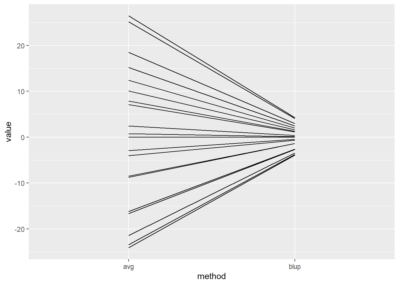
Sometimes the units that form the grouping are of interest. In this specific case the cages may not be our primary focus of attention, but sometimes it could be. In the frame work of mixed models evaluations of those groups are a combination of the actual observations within those groups and the fact they belong to a distribution described by all other groups in the data set. So for each cage we have a prediction rather than the pure estimate (i.e only corrected for the fixed effect of supplier) In the case of mixed models these are called a blup (best unbiased prediction).

For a lme4-model object we can obtain them via:

ranef(modlmer.1.0)
$cage
        (Intercept)
cage1   0.009037572
cage10  2.441148560
cage11  0.125521831
cage12 -3.450344077
cage13  1.145763269
cage14 -1.366681691
cage15  4.043811292
cage16  1.270280925
cage17  4.249667094
cage18  1.997303367
cage19  0.388615587
cage2  -3.767663265
cage20 -2.607841551
cage3  -2.674117077
cage4   1.621742050
cage5  -3.877118301
cage6  -1.404840327
cage7   2.968340248
cage8  -0.468949559
cage9  -0.643675947

with conditional variances for "cage" 

These blups are shrunken compared to the estimates as can be seen in the graph below that compares the raw means of the cages with their blups. This shrinkage is the result of the combination of the data of the specific cage and the fact that is should fit within the framework of hierarchies and the behaviour within the other cages.

# blups are 'shrunken'
compareRF <- data.frame(blup=ranef(modlmer.1.0)$cage[,1], 
           data.frame(cage=chickensC$cage,resfe=residuals(modlm.1.0)) %>% 
             group_by(cage) %>% 
             summarise(avg=mean(resfe)))

compareRF %>% 
  pivot_longer(cols=c(blup,avg),names_to = "method") %>%
  ggplot(aes(y=value,x=method,group=cage)) + geom_line()

More examples of this shrinkages will be seen later on in more complex models.

2.5 On the side: the Z matrix

For those who like to see how the Z matrix looks like:

getME(modlmer.1.0,"Z") %>% as.matrix()
   cage1 cage10 cage11 cage12 cage13 cage14 cage15 cage16 cage17 cage18 cage19
1      1      0      0      0      0      0      0      0      0      0      0
2      1      0      0      0      0      0      0      0      0      0      0
3      1      0      0      0      0      0      0      0      0      0      0
4      1      0      0      0      0      0      0      0      0      0      0
5      0      0      0      0      0      0      0      0      0      0      0
6      0      0      0      0      0      0      0      0      0      0      0
7      0      0      0      0      0      0      0      0      0      0      0
8      0      0      0      0      0      0      0      0      0      0      0
9      0      0      0      0      0      0      0      0      0      0      0
10     0      0      0      0      0      0      0      0      0      0      0
11     0      0      0      0      0      0      0      0      0      0      0
12     0      0      0      0      0      0      0      0      0      0      0
13     0      0      0      0      0      0      0      0      0      0      0
14     0      0      0      0      0      0      0      0      0      0      0
15     0      0      0      0      0      0      0      0      0      0      0
16     0      0      0      0      0      0      0      0      0      0      0
17     0      0      0      0      0      0      0      0      0      0      0
18     0      0      0      0      0      0      0      0      0      0      0
19     0      0      0      0      0      0      0      0      0      0      0
20     0      0      0      0      0      0      0      0      0      0      0
21     0      0      0      0      0      0      0      0      0      0      0
22     0      0      0      0      0      0      0      0      0      0      0
23     0      0      0      0      0      0      0      0      0      0      0
24     0      0      0      0      0      0      0      0      0      0      0
25     0      0      0      0      0      0      0      0      0      0      0
26     0      0      0      0      0      0      0      0      0      0      0
27     0      0      0      0      0      0      0      0      0      0      0
28     0      0      0      0      0      0      0      0      0      0      0
29     0      0      0      0      0      0      0      0      0      0      0
30     0      0      0      0      0      0      0      0      0      0      0
31     0      0      0      0      0      0      0      0      0      0      0
32     0      0      0      0      0      0      0      0      0      0      0
33     0      0      0      0      0      0      0      0      0      0      0
34     0      0      0      0      0      0      0      0      0      0      0
35     0      0      0      0      0      0      0      0      0      0      0
36     0      0      0      0      0      0      0      0      0      0      0
37     0      1      0      0      0      0      0      0      0      0      0
38     0      1      0      0      0      0      0      0      0      0      0
39     0      1      0      0      0      0      0      0      0      0      0
40     0      1      0      0      0      0      0      0      0      0      0
41     0      0      1      0      0      0      0      0      0      0      0
42     0      0      1      0      0      0      0      0      0      0      0
43     0      0      1      0      0      0      0      0      0      0      0
44     0      0      1      0      0      0      0      0      0      0      0
45     0      0      0      1      0      0      0      0      0      0      0
46     0      0      0      1      0      0      0      0      0      0      0
47     0      0      0      1      0      0      0      0      0      0      0
48     0      0      0      1      0      0      0      0      0      0      0
49     0      0      0      0      1      0      0      0      0      0      0
50     0      0      0      0      1      0      0      0      0      0      0
51     0      0      0      0      1      0      0      0      0      0      0
52     0      0      0      0      1      0      0      0      0      0      0
53     0      0      0      0      0      1      0      0      0      0      0
54     0      0      0      0      0      1      0      0      0      0      0
55     0      0      0      0      0      1      0      0      0      0      0
56     0      0      0      0      0      1      0      0      0      0      0
57     0      0      0      0      0      0      1      0      0      0      0
58     0      0      0      0      0      0      1      0      0      0      0
59     0      0      0      0      0      0      1      0      0      0      0
60     0      0      0      0      0      0      1      0      0      0      0
61     0      0      0      0      0      0      0      1      0      0      0
62     0      0      0      0      0      0      0      1      0      0      0
63     0      0      0      0      0      0      0      1      0      0      0
64     0      0      0      0      0      0      0      1      0      0      0
65     0      0      0      0      0      0      0      0      1      0      0
66     0      0      0      0      0      0      0      0      1      0      0
67     0      0      0      0      0      0      0      0      1      0      0
68     0      0      0      0      0      0      0      0      1      0      0
69     0      0      0      0      0      0      0      0      0      1      0
70     0      0      0      0      0      0      0      0      0      1      0
71     0      0      0      0      0      0      0      0      0      1      0
72     0      0      0      0      0      0      0      0      0      1      0
73     0      0      0      0      0      0      0      0      0      0      1
74     0      0      0      0      0      0      0      0      0      0      1
75     0      0      0      0      0      0      0      0      0      0      1
76     0      0      0      0      0      0      0      0      0      0      1
77     0      0      0      0      0      0      0      0      0      0      0
78     0      0      0      0      0      0      0      0      0      0      0
79     0      0      0      0      0      0      0      0      0      0      0
80     0      0      0      0      0      0      0      0      0      0      0
   cage2 cage20 cage3 cage4 cage5 cage6 cage7 cage8 cage9
1      0      0     0     0     0     0     0     0     0
2      0      0     0     0     0     0     0     0     0
3      0      0     0     0     0     0     0     0     0
4      0      0     0     0     0     0     0     0     0
5      1      0     0     0     0     0     0     0     0
6      1      0     0     0     0     0     0     0     0
7      1      0     0     0     0     0     0     0     0
8      1      0     0     0     0     0     0     0     0
9      0      0     1     0     0     0     0     0     0
10     0      0     1     0     0     0     0     0     0
11     0      0     1     0     0     0     0     0     0
12     0      0     1     0     0     0     0     0     0
13     0      0     0     1     0     0     0     0     0
14     0      0     0     1     0     0     0     0     0
15     0      0     0     1     0     0     0     0     0
16     0      0     0     1     0     0     0     0     0
17     0      0     0     0     1     0     0     0     0
18     0      0     0     0     1     0     0     0     0
19     0      0     0     0     1     0     0     0     0
20     0      0     0     0     1     0     0     0     0
21     0      0     0     0     0     1     0     0     0
22     0      0     0     0     0     1     0     0     0
23     0      0     0     0     0     1     0     0     0
24     0      0     0     0     0     1     0     0     0
25     0      0     0     0     0     0     1     0     0
26     0      0     0     0     0     0     1     0     0
27     0      0     0     0     0     0     1     0     0
28     0      0     0     0     0     0     1     0     0
29     0      0     0     0     0     0     0     1     0
30     0      0     0     0     0     0     0     1     0
31     0      0     0     0     0     0     0     1     0
32     0      0     0     0     0     0     0     1     0
33     0      0     0     0     0     0     0     0     1
34     0      0     0     0     0     0     0     0     1
35     0      0     0     0     0     0     0     0     1
36     0      0     0     0     0     0     0     0     1
37     0      0     0     0     0     0     0     0     0
38     0      0     0     0     0     0     0     0     0
39     0      0     0     0     0     0     0     0     0
40     0      0     0     0     0     0     0     0     0
41     0      0     0     0     0     0     0     0     0
42     0      0     0     0     0     0     0     0     0
43     0      0     0     0     0     0     0     0     0
44     0      0     0     0     0     0     0     0     0
45     0      0     0     0     0     0     0     0     0
46     0      0     0     0     0     0     0     0     0
47     0      0     0     0     0     0     0     0     0
48     0      0     0     0     0     0     0     0     0
49     0      0     0     0     0     0     0     0     0
50     0      0     0     0     0     0     0     0     0
51     0      0     0     0     0     0     0     0     0
52     0      0     0     0     0     0     0     0     0
53     0      0     0     0     0     0     0     0     0
54     0      0     0     0     0     0     0     0     0
55     0      0     0     0     0     0     0     0     0
56     0      0     0     0     0     0     0     0     0
57     0      0     0     0     0     0     0     0     0
58     0      0     0     0     0     0     0     0     0
59     0      0     0     0     0     0     0     0     0
60     0      0     0     0     0     0     0     0     0
61     0      0     0     0     0     0     0     0     0
62     0      0     0     0     0     0     0     0     0
63     0      0     0     0     0     0     0     0     0
64     0      0     0     0     0     0     0     0     0
65     0      0     0     0     0     0     0     0     0
66     0      0     0     0     0     0     0     0     0
67     0      0     0     0     0     0     0     0     0
68     0      0     0     0     0     0     0     0     0
69     0      0     0     0     0     0     0     0     0
70     0      0     0     0     0     0     0     0     0
71     0      0     0     0     0     0     0     0     0
72     0      0     0     0     0     0     0     0     0
73     0      0     0     0     0     0     0     0     0
74     0      0     0     0     0     0     0     0     0
75     0      0     0     0     0     0     0     0     0
76     0      0     0     0     0     0     0     0     0
77     0      1     0     0     0     0     0     0     0
78     0      1     0     0     0     0     0     0     0
79     0      1     0     0     0     0     0     0     0
80     0      1     0     0     0     0     0     0     0